Before I proceed any further with any design, I need to do parametric sweeps and save/export the results and get proper graphs that I can use forever. I’ve done parametric sweeps before but I usually restrict them to a narrow range or keep a few things fixed and re-run as needed. I hate programming and scripting but I love circuits, so I just close my eyes and think of an LNA while I write OCEAN scripts or whatever.

I also don’t know Cadence’s syntax. There’s all sorts of weird little quirks, and it’s changed over the years. ADE L is pretty much discontinued and you now have to use Maestro, but that’s a recent change so most every tutorial is out of date.

After a ton of messing around with different test setups and learning OCEAN scripting — like literally a full weekend of messing with OCEAN scripts — the method below is what I’ve found to be the best mix of comprehensive while also being simple. Full gm/Id sweeps supposedly take like 2-3 days to run, and they throw a *ton* of data at you, much of which is not actually useful and it becomes time consuming to work through. I’m not working with FinFETs here or doing crazy subthreshold low power design, so I’m just doing what works for student/hobbyist use and not anything cutting edge.

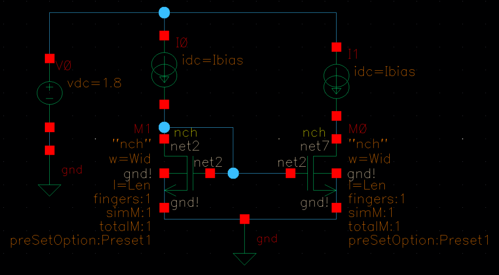
I also ran into issues where sweeping through gate voltages and bias currents kept getting evaluation errors because certain combinations didn’t work. The solution to that is to make the MOSFET diode connected but then you’re not getting an accurate reflection of the transistor when it’s below or near saturation. Therefore I used the test setup shown below to get data that correlates to how transistors will actually be biased in operation. For example in an OTA, the current mirror load is current biased by the tail current of the OTA but its gate is biased by a current mirror. *That’s* the situation I want to capture.

The schematic below is my test setup. All data will be collected from M0, the DUT.

Here’s what my ADE Explorer setup looks like, the expressions I’m plotting. Notice how I first get wt, and then I have to make a separate expression to convert it from radians/second to Hz (Cgs is a negative value so it’s multiplied by -1). Also notice that the W/L ratio is its own separate line, pulled out as VAR( ) expressions. All these things have to be separated out this way for some reason. If I’m doing this wrong and someone knows how to combine these things please let me know in the comments.

I’m running Ibias from 100nA to 4mA logarithmically, and stepping the Width from 5um to 500um logarithmically. I’ve found that this gives me the most useful results and satisfies my need for giving me enough data to be useful but not overwhelmingly so. It’s a small enough amount of data that I can just keep this setup in a separate window and re-run simulations as needed to get more precise values. Here’s a sample set of graphs for when the Length is 200nm.

I’ve graphed:

• gm/Id vs Ibias
• rds vs Ibias
• Vdsat vs Ibias
• Intrinsic gain (gm*rds) vs Ibias
• Transition frequency vs gm/Id
• Transition frequency vs Ibias

I’ve run this for a few different lengths ranging from 60nm (the lowest possible for the 65nm node) up to 1um. I add markers and save the images so I can use them later, but I also know that I have this available in case I need it.

For those of you who do want to go down the route of scripting, I followed this incredibly helpful guide at this link.

Quick caveat, the “close(file)” gives an error (“close: argument #1 should be an I/O port (type template = “p”) – nil”) if the file open is invalid/nil, which happens if the folder doesn’t exist. So if you want to save to ./Curves/gmByIdCurves.csv like it says, you have to create the Curves folder, it won’t create it for you. I don’t know if this is a typical Linux feature, but it caught me up for a while.