Hi everyone! Today I wanted to talk about poles and zeros, what they are mathematically, but more importantly provide intuition for what they actually represent in a circuit, and why it’s so much easier to find and approximate poles while most textbooks either ignore zeros or “predict” them.

An excellent text that helped me connect a signals/systems understanding with practical circuits and power applications is Designing Control Loops For Linear and Switching Power Supplies by Christophe Basso. Any of his texts on design, analysis, or simulation are worthwhile reads.

Transfer Functions

A circuit can be infinitely complex inside, but it can be abstracted all the way up to a very simple box, with an input and an output. When we source a voltage or current into the input, we can expect a certain voltage or current at the output. Rather than outlining a list of all possible combinations, we can just write it as a ratio. That ratio is the transfer function.

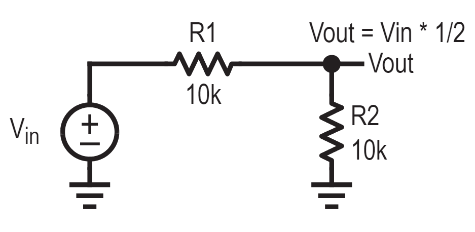
The circuit below should be familiar, it’s a simple voltage divider. This is about as simple of a transfer function as you can get. The output is half the input. The transfer function is simply 1/2, super easy.

If we replace the lower resistor with a capacitor, we’ve added some complication. Unlike a resistor which dissipates energy as heat, a capacitor stores and releases energy.

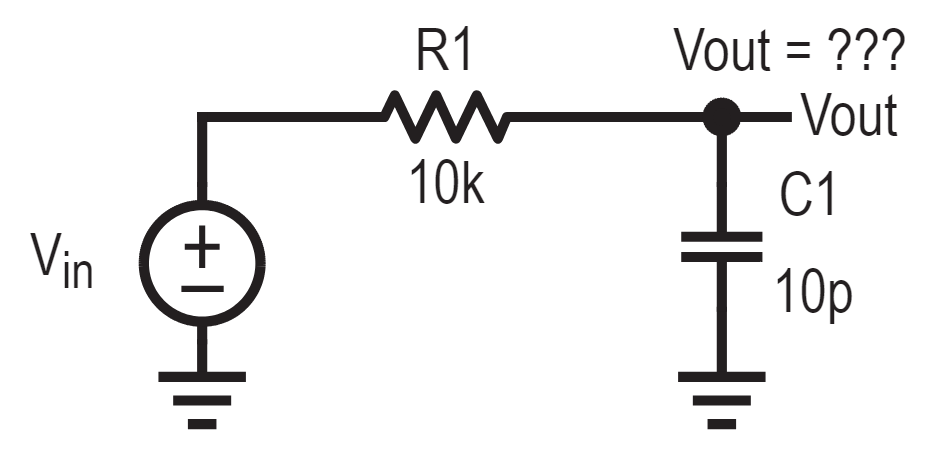
Because of the pesky laws of the universe, energy can’t be created or destroyed in an instant, it has to be stored or released over time. Even if it’s nanoseconds, it’s still some amount of time. In the context of sine waves, time translates to frequency and phase. Higher frequency means less time to respond, and if you have a device that can only store energy so fast, then as the frequency increases the device has a harder time keeping up.

If we get smart and use our nifty gifty Laplace transform we can avoid gross differential equations and just use algebra. Sounds counterintuitive, but the complex Laplace transform actually keeps things easy and lets us stick to the physics and concepts instead of getting lost in calculus-land. From an algebra perspective, the capacitor and resistor are still a voltage divider.

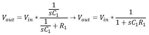
Our transfer function is now not just a number, but is dependent on this “s” variable — a representation of oscillations and transients. As we add capacitors and inductors, more “s” variables are getting multiplied in, and we develop polynomials. To learn more about the s-domain, read our page about imaginary numbers and visualizing the s-plane.

Numerator and Denominator

Regardless of how complicated it gets, the transfer function is nothing more than a ratio between two polynomials, a numerator and denominator. Whenever we see a polynomial, our instinct should be to solve it i.e. find its roots. Finding the roots of a polynomial can give us some useful information.

Even though we’re in the s-domain, it’s the same algebra you learned in high school, same rules apply. We like to get it into the form below, and the roots of each polynomial become apparent.

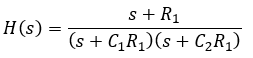
The roots of the numerator are known as zeros and the roots of the denominator are known as poles. They’re called that because if one of those numerator terms is zero, then the whole numerator is zero, which means the whole transfer function is zero; for the denominator, if one of the terms is zero, you’re now dividing by zero and you’ve got an asymptote to infinity.

(Quick note on why they’re called poles: it actually originally comes from cartography and the north/south pole. Magnets point to the north pole, so that’s the point of reference. If you pick any spot on a globe, there is always one unique shortest path to the north pole. Except for the south pole. At the south pole, there are an infinite number of shortest paths to the north pole. This asymptotic explosion to infinity is how poles got their name.)

Circuits: All Naturale

What do poles and zeros mean in a circuit? It’s just a bunch of algebra and numbers right now, what does that have to do with these physical components? Like, if you buy an inductor off Digikey for 5 cents and add it to your circuit, you’ve physically changed it but you’ve also modified its polynomials? What does that even mean? There needs to be some way to consolidate these perspectives.

It’s all about the energy storage. No matter how abstract you get, whether you’re talking about differential equations, or the s-domain, or transfer functions, it comes back to storing energy as an electric or magnetic field.

Zeros

For our linear circuit, the box with an input and output, the numerator tells us around what frequencies the input doesn’t reach the output, leaving it at zero. Some examples are shown below.

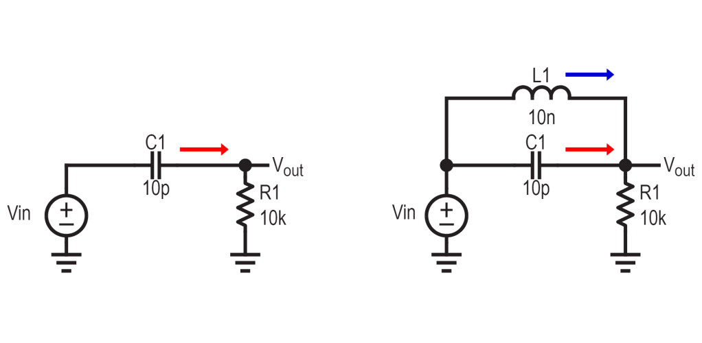
In the circuit on the left, when the frequency is low, the capacitor is being a huge pain in the ass, so the resistor pulls the output low. That’s a “zero”.

In the circuit on the right, however, the inductor provides an alternate path around the capacitor. As we increase the frequency, the capacitor is more reasonable but at super higher frequencies the inductor becomes a pain in the ass. If we go back down, at juuuuust the right sweet spot in the middle, both the inductor and capacitor are being equally difficult. Once again, the resistor dominates and pulls the output low. This means we have a zero at some finite frequency, and now it appears in our transfer function.

That’s it, that’s a zero. Input not arriving at output? Zero. That’s mathematically represented by the numerator of the transfer function. This is also known as the forced response because it’s the response of the system when you force energy into it.

Poles

Poles don’t have a concept of inputs or outputs. Poles are about what happens when there is no input, which is why it’s represented by the unforced/natural response. It’s a hypothetical. Look at just the circuit and only the circuit. We’re not inputting anything, but the energy storage elements have some energy already in them. What happens then? That latent energy, electric or magnetic, will naturally release and dissipate through the resistors in the form of heat.

In other words, the circuit itself is the input. Each energy storage element, capacitor or inductor, acts as a source, with the rest of the circuit as the load. As a result, finding poles lends itself very well to analysis by inspection. That’s the fancy term for when you can just look at it and kinda figure it out. Generally speaking, there are as many poles as there are energy storing devices. If you have an inductor and a capacitor, you can easily say there are two poles.

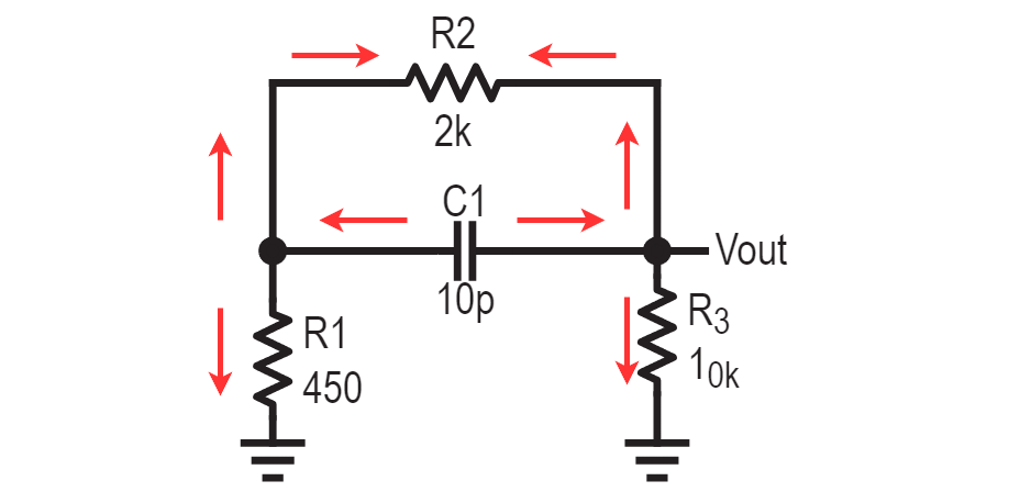
There are some exceptions, like when a capacitor is flanked by capacitors on either end. In the circuit below, your gut instinct (the one you learned 5 seconds ago) might tell you there are three poles because there are three capacitors. But in this scenario, only two of the capacitors have unique energy storage values.

If we were to hypothetically say that C1 has a charge of 1nC, and that C3 has a charge of 5nC, by the equation Q=CV, you have voltages at node A and B. This fixes a voltage across C2 and automatically determines its charge. C2 cannot have an arbitrary hypothetical charge of its own, it’s not independent.

By inspection, we can say the number of poles is the number of independent initial conditions. That’s voltages across capacitors, and currents through inductors. Other than special cases like the one above, this is super easy to find, just count the numbers of capacitors and inductors and you’re good.

Positive Feedback: Not Just The Name Of This Blog

You may have heard in passing about how poles are dangerous or zeros cause instability or whatever the hell. Why are poles and zeros an issue? The answer is amplifiers and feedback.

Amplifiers look at their inputs, and then output something based on that input. That output is coming from the power source. Amplifiers aren’t creating energy from nothing, they’re not transforming the input into an output. They’re directing energy in from an external source to give the illusion of making the input bigger.

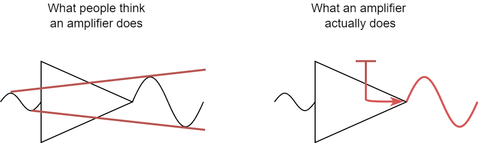
Amplification is a good thing, but electronic amplifiers are imprecise and unpredictable. They’re a cacophony of physics and god knows what little gremlins reside within the hallowed halls of those silicon bastards. To make an amplifier work reliably, there needs to be some sort of feedback mechanism that keeps it from getting out of control.

Our feedback loop might involve some energy storage, either on purpose because we want it to be frequency-dependent, or by accident. If you buy an op-amp and put it onto a PCB, you are adding parasitic capacitors and inductors whether you want to or not, just because of the package leads.

If we take the op-amp above and put it into a standard inverting amplifier configuration, we might actually be creating a slightly different circuit because of the parasitics. Zeros and poles have been added just from the physical construction.

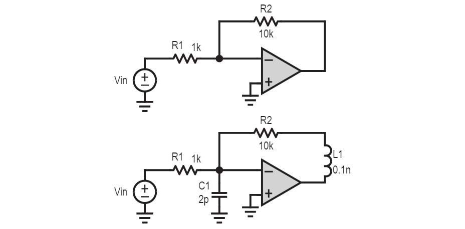
Think about this series of events for the configuration below. The amplifier sees a voltage at its input and outputs a current. This current goes through its feedback back to its input. At the input is a capacitor, which gets charged up by this current, increasing its voltage. That voltage gets amplified, and so on.

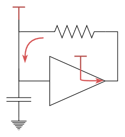
This is a recipe for disaster, an endless positive feedback loop. The capacitor will also naturally discharge through the resistor, but if the capacitor is charged faster than it discharges, then the amplifier’s output gets bigger and bigger instead of stabilizing. The path for dissipating energy is also the mechanism for injecting energy back in???? Straight to jail. The output may rail high or low or oscillate between the two. So if we have any sort of poles or zeros with gain/amplification, we have to be careful. Maybe our output doesn’t get fed back to the input, or that the amplification blows itself up.

The Quest(love) for the Roots

Okay so we understand poles and zeros as being physically related to pathways of energy transfer and dissipation, and mathematically related to the roots of an algebraic equation, but how do we use them? How do we find them?

Let’s go over some of the tools we have to get the transfer function and identify poles and zeros.

a. KVL/KCL

This is the brute force method. You set up your equations, you set up your equations, find Vout as a function of Vin, and then factor out the resulting equation. This way works. This way is tedious.

b. Modified Nodal Analysis (MNA)

This method is based on KVL/KCL but more algorithmic. You don’t need to identify loops or even nodes, you just go component by component, and add it to a matrix (called “stamping”). This site has a great writeup on how to go through an MNA algorithm.

It’s unwieldy, but because it’s a matrix that can be analyzed with an algorithm, it’s perfect for computers. Modified Nodal Analysis is in fact the very basis of all circuit simulators such as SPICE.

To find poles, you take the determinant of the matrix, whereas the zeros are found by taking the determinant of the matrix in which the matrix minor (the relevant column/row combo) is replaced with the source and output voltage and current variables.

May not be useful to us for actually deriving anything, but it reveals a lot about the nature of poles and zeroes in circuits. If you enter a circuit into a matrix through Modified Nodal Analysis, that circuit in and of itself reveals its own poles, just take the determinant, no adjustments required. Put more simply, a pole anywhere is a pole everywhere. To find the zeroes, you have to specify the input and output nodes, and replace those rows/columns in the matrix accordingly, and then do the math.

c. Driving Point Impedance + Short Circuit Current

This is a more….humane way of doing KVL/KCL. I like to think of it like I’m “folding” a circuit inward, from source to load. Like these guys.

In the example below, we look at the node between R1 and R2, and ignore everything to the right of it. Very similar to finding the Thevenin equivalent, we find the current through a hypothetical wire that short-circuits the node we care about while the input is then, then find the apparent resistance if we were to shut off the input but put a voltage source at the output instead.

In this scenario, if we tie a wire from Vx to ground, all the current going through R1 would go through it since it shorts out R2. That current, by Ohm’s Law, is just Vin/R1. That’s our “short-circuit current”. Let’s remove that wire, and replace it with a voltage source of our own. If we turn off Vin, now the other side of R1 is 0V i.e ground. That makes R1 and R2 in parallel, which is R1*R2/(R1+R2). That’s the driving-point-impedance (DPI). Multiply the two together and you get the voltage at that node. In this case it’s a simple voltage divider, which we probably could have easily guessed, but for circuits with even a slightly bit more complexity, this method lets us tackle it piece by piece while still respecting the rules of KVL/KCL.

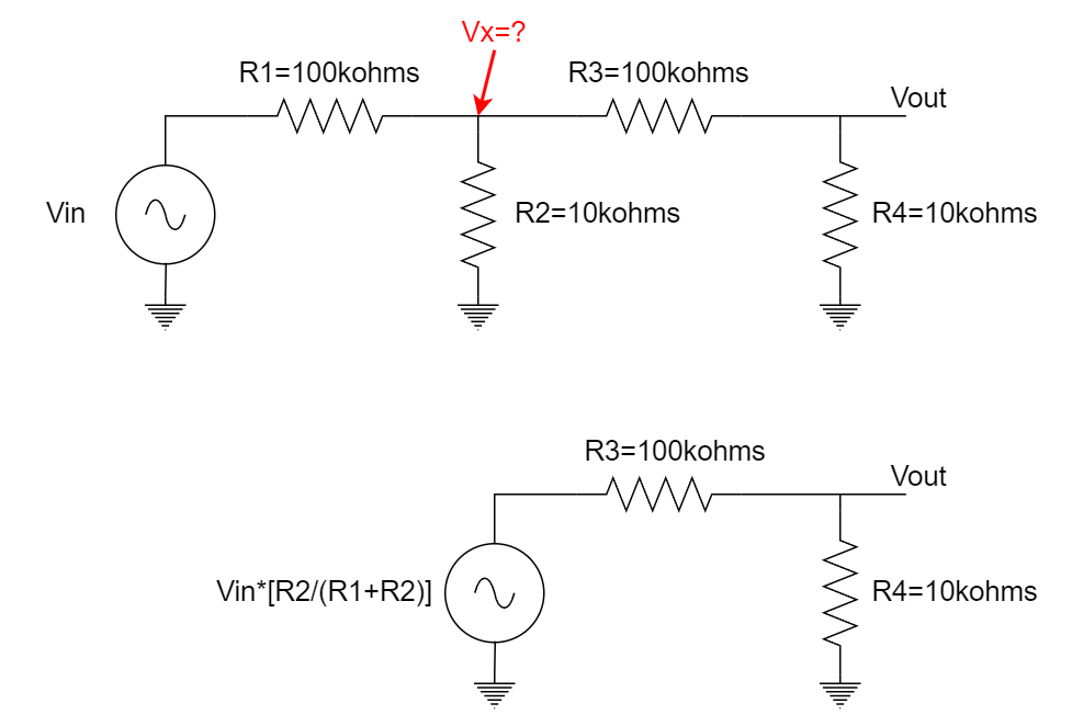
We analyze each piece and fold it into a new voltage source until we get our final output, which gets us an equation that is not only accurate but also revealing. We can get a numerical value, or we can keep it analytical, and can even keep components as “R1 in parallel with R2” rather than multiplying it out. It lets us see what components and values actually matter and affect the final outcome.

Professor Johns has a great video on this rapid hand-analysis technique. This is the one I personally use the most and is frequently used in microelectronics. The concepts lend themselves to creating signal flow graphs/block diagrams, a very powerful tool that can provide lots of insight while also being useful in actually creating designs.

d. Null Double Injection

This is a tricky concept to grasp, but once you get it can be used with great success. It was a technique developed and pioneered by Dr. Middlebrook of Caltech, the “inventor” of power electronics.

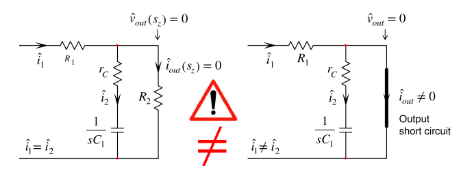
Poles are found by looking at the impedance seen from the perspective of each capacitor/inductor while the input is off. For a zero though, it’s more complex. What we do is we keep the input on, but we also set the output voltage and the output current to zero (we call this a NULL to distinguish it from just being a short circuit as shown below), and then replace the capacitor/inductor with a current source. We find if there is a frequency at which that new current source can make the output voltage and current zero.

Null Double Injection also provides a quick inspection technique: to see if a capacitor/inductor has a zero associated with it, short the capacitor or open the inductor and see if a response still exists. If there is still a response, then the capacitor/inductor adds a zero to the transfer function. This is a way bigger qualifier than when we found poles by inspection, which amounted to “just look at the damn thing”.

So once again, we see poles are about how energy is dissipated by capacitors and inductors in the absence of a source, while zeros are about how that energy dissipation prevents a source from reaching its destination.

e. Extra Element Theorem

Another great one from Dr. Middlebrook. The idea is this: if there’s a component that’s giving us trouble, why not just remove it and analyze everything else, then modify that transfer function? It uses ideas brought up in this page already, like the driving point impedance (DPI) and null double injection (NDI) but can be generalized to much larger circuits.

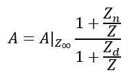
We find three quantities. First is the transfer function A-Z-infinite when the extra element is infinite — short circuit capacitor or open circuit inductor. Next we remove the extra element, Z, giving us an open port we can look into. The second quantity is the impedance seen at this open extra element port, called Zd. The third quantity is the impedance seen here when the output is nulled (zero voltage and zero current), called Zn. We combine them together to create an overall transfer function, which we can factor to get our zeros and poles.

The EET can be generalized up to what is known as the N-EET, which is for higher order systems, where you can remove an arbitrary N number of extra elements. It’s somehow even further generalized by Professor Hajimiri’s General Time and Transfer Constant method, which combines the N-EET the open-circuit time-constant and zero-value time constant (two ways of finding the overall bandwidth instead of the exact location of every pole/zero).

Honestly, these aren’t worth really going into unless you’re doing some crazy mixed-signal/RF IC research, they sort of circle back around to being as tedious as brute-forcing it with KVL and KCL.

Conclusion

Poles and zeros tell us how energy flows — or doesn’t flow — in a circuit. Poles tell us how energy flows without an input, agnostic to specific paths and structures, while zeros tell us how energy flows from the input to the output and how it might be blocked.

They represent a circuit’s mathematical transfer function, but they also represent physical storage and transfer of electric/magnetic fields by circuit components. They can be used as tools to block or permit certain frequencies, but the energy storage can also destabilize amplifiers when placed incorrectly in a feedback loop, whether on purpose or by accident.

There are multiple tools to find them, with varying degrees of usefulness for a given situation. MNA is best for a computer, but Null Double Injection might be better for pen-and-paper design. Driving point impedance might be more appropriate for CMOS design, while Extra Element Theorem provides a clearer picture for power electronics.

The methods themselves show us that poles are derived entirely from the circuit’s structure, whereas zeros depend on what you consider the input and output, which makes them harder to find.

Well that’s enough stressful equations and circuits for the day. Time to relax and ball out.

• Uncategorized