This is a write-up of a really fun problem I solved at at Lake Shore Cryotronics, originally written as a presentation I did for my job at Bruker. I love circuits as my 9-5 job, but I do get a high from doing silly math or improving some multi-rate DSP thing here and there. This seemed like a solved problem but I couldn’t find anything about this online which had me wicked frustrated, because I hate reading; I’m putting up my solution here so nobody else has to endure the suffering of some light googling.
The main idea is that if you’re using a digital high pass filter to get rid of the DC component, it will make the DC component zero, but your signal of interest will also be attenuated. This is how to calculate a gain factor to un-attenuate your signal so you can block the DC component and leave your signal unharmed (you can skip to the bottom if you just want the answer).
Lock-In Amplifier
The purpose of lock-in amplification is to measure very low values in the presence of noise. It’s important to understand that the parameter being measured is a quote-unquote DC value. For example, we may be trying to characterize the nominally static carrier mobility of some novel semiconductor device, and measuring nanovolts using excitation in the femto- or picoamp range.
The method is as follows:
- Excite the DUT with a precisely controlled sinusoid on the source side. Excitation can be current or voltage.
- Measure the DUT’s current or voltage.
- Produce two sinusoids, 90 degrees phase shifted from each other, internal to the measurement device (I and Q), of the exact same frequency as the source. If the source and measure are coming from different devices, the source should have a way to output its frequency to the measure device.
- Multiply the incoming signal by the I and Q sinusoids to get an X and Y value
- Apply filters (usually a moving average, followed by a simple 2 or 3 pole IIR)
- Calculate the magnitude and phase from the filtered X and Y

This provides some advantages. The image below shows a signal, and the same signal buried in noise. The lock-in amplifier can get you the magnitude and phase of the signal of interest with ease in both situations.
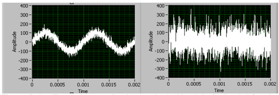
The key is that it’s being purposely modulated and then purposely synchronously demodulated with the exact same frequency in the time domain. When it’s modulated by the source by frequency F, the DC parameter is multiplied by a cosine with frequency F and so the resulting frequency spectrum is a spike at F, with noise throughout as well as a DC portion, as shown on the left.
The measurement side then multiplies it by a sinusoid. When you multiply one sinusoid of frequency F1 by another of frequency F2, the result is two sinusoids, one of frequency F1-F2 and another of F1+F2. If F1 and F2 are matched, which they will be with a lock-in amplifier because F1 is being directly sent to the measurement device where it’s reproduced by an oscillator, then the F1-F2 wave becomes a sinusoid with frequency 0 i.e a perfect DC signal.
We can then apply sharp narrowband filters to get rid of all the unwanted noise. All of this is done in real time in the time domain, providing great performance with relatively little processing power. As a reference, our latest measurements showed a total noise of ~3.2nV RMS.
DC Blocker
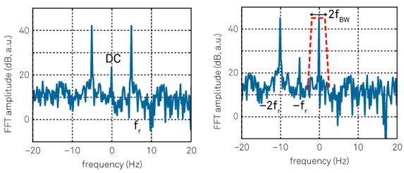
When putting out the excitation, the user may want to apply a DC bias to the DUT, and then see its characteristics at that operating point. A very common application is semiconductors, where you’re applying a forward bias and seeing its behavior. This means there’s now a DC component on the measurement. The issue this introduces is that when the signal is demodulated by multiplying F1 by F2, the DC bias also gets shifted up. F1 gets shifted down to DC, but DC gets shifted up to F1. Even when filtered out it may produce an unacceptable error.
Our solution to this was to use a digital high-pass filter, which would outright fully block any DC component, before demodulating. This high-pass filter would also attenuate the signal itself, because a high pass filter isn’t 1 until the max frequency, so we would need to apply gain correction (simply the inverse of the transfer function) to retrieve the correct value.
This needed to happen in the pre-processing, where there’s very few resources remaining. By resources I’m talking in terms of single-digit clock cycles. In order to reduce clock cycles to implement the filter, rather than figuring out the actual “alpha” value by which to multiply the signal to filter, we would simply do a bit shift to divide. A multiply instruction takes several clock cycles, while shifting the bits to the right is a single clock cycle.
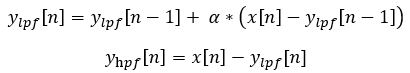
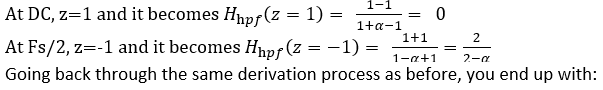
The simple way to create a high-pass filter is to create a low-pass filter, and then subtract that from the input. In the time domain it looks like the following:
The z-transform of this difference equation is
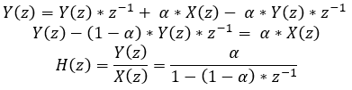

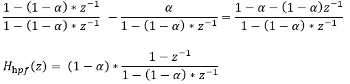
What’s interesting about this is that while it does block DC (it outputs 0 when z=1), at the Nyquist frequency Fs/2 (z=-1) it attenuates the signal to 2*(1-a)/(2-a).


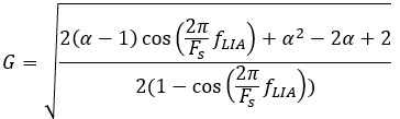
Substituting everything back in, the final gain correction that should be applied to a frequency given a certain alpha is

The New Problem
This seemed to work, in that adding a DC bias and changing its value experiment to experiment didn’t affect the results in an unexpected way. But when the application scientists performed experiments that never required the DC bias in the first place, they found that the results were now off.
Examination of the code found out that in an effort to minimize clock cycles, rather than using the low pass to create the high pass, whoever implemented it found a recursive trick and created the low pass using the high pass, reducing the number of instructions. But by doing so they didn’t realize that the next high pass index would be using the previous low pass index, when what we want to do is use the current low pass index. Mathematically, our new time-domain equation becomes:

It’s a subtle difference but compare it to what we found it should be in the previous section. The ylpf[n] is now off by 1. Delaying something by 1 in the time domain is the same as multiplying by 1/z in the z-domain. The new transfer function in the z-domain therefore becomes:

The only difference was the 1/(1-a) term. We experimentally confirmed that all the new results were being gained up by an extra 1-a. Once we removed that part of the gain correction, everything was fixed! Yay!
Obligatory Giuseppe picture:

